SPAM timeseries
SPAM recordings are more complex than ATS recordings. Continuous recordings can either be stored in a single data file or multiple smaller data files. All channels are in the same data file.
Therefore, a typical SPAM data directory can look like this,
run01
├── 0996_LP00100Hz_HP00000s_R016_W038.XTR
└── 0996_LP00100Hz_HP00000s_R016_W038.RAW
or this,
run02
├── 0996_LP00100Hz_HP00000s_R016_W079.XTR
├── 0996_LP00100Hz_HP00000s_R016_W079.RAW
├── 0996_LP00100Hz_HP00000s_R016_W080.XTR
├── 0996_LP00100Hz_HP00000s_R016_W080.RAW
├── 0996_LP00100Hz_HP00000s_R016_W081.XTR
└── 0996_LP00100Hz_HP00000s_R016_W081.RAW
as long as together, the recordings are continuous and without gaps.
Warning
Resistics requires that each data folder represents a continuous recording without gaps. If gaps are encountered, resistics will quit execution and state where gaps were encountered.
Note
In order for resistics to recognise a SPAM data folder, the following have to be present:
A header file with extension .XTR or .XTRX
Data files with extension .RAW
Note that .XTRX headers are not yet supported. But where a .XTRX header is present, header information is read from the header of the binary data file.
Note
Unscaled units for SPAM data are as follows:
All channels are floats in mV
Raw SPAM timeseries data in the data files is in Volts. However, some scaling is applied to give “unscaled” data in mV. The reason for this is due to varying gains between SPAM data files, even when they together constitute a single continuous recording. Therefore, for the data to make sense as a single data source, gains are removed, leaving “unscaled” data in mV. When getting “physical” samples, electric channels are further divided by the electrode spacing in km.
SPAM recordings are opened in resistics using the TimeReaderSPAM class. An example is provided below:
1 2 3 4 5 6 7 | from datapaths import timePath, timeImages
from resistics.time.reader_spam import TimeReaderSPAM
# read in spam data
spamPath = timePath / "spam"
spamReader = TimeReaderSPAM(spamPath)
spamReader.printInfo()
|
spamReader.printInfo() prints the measurement information out to the terminal and displays various recording parameters.
1 2 3 4 5 6 7 8 9 10 11 12 13 14 15 16 17 18 19 20 21 22 23 24 | 13:51:34 DataReaderSPAM: ####################
13:51:34 DataReaderSPAM: DATAREADERSPAM INFO BEGIN
13:51:34 DataReaderSPAM: ####################
13:51:34 DataReaderSPAM: Data Path = timeData\spam
13:51:34 DataReaderSPAM: Global Headers
13:51:34 DataReaderSPAM: {'sample_freq': 250.0, 'start_date': '2016-02-07', 'start_time': '00:00:00.003200', 'stop_date': '2016-02-07', 'stop_time': '23:59:59.999200', 'num_samples': 21600000, 'ats_data_file': '0996_LP00100Hz_HP00000s_R016_W038.RAW', 'meas_channels': 4}
13:51:34 DataReaderSPAM: Channels found:
13:51:34 DataReaderSPAM: ['Hx', 'Hy', 'Ex', 'Ey']
13:51:34 DataReaderSPAM: Channel Map
13:51:34 DataReaderSPAM: {'Hx': 0, 'Hy': 1, 'Ex': 2, 'Ey': 3}
13:51:34 DataReaderSPAM: Channel Headers
13:51:34 DataReaderSPAM: Hx
13:51:34 DataReaderSPAM: {'gain_stage1': 1, 'gain_stage2': 1, 'hchopper': 1, 'echopper': 0, 'ats_data_file': '0996_LP00100Hz_HP00000s_R016_W038.RAW', 'num_samples': 21600000, 'sensor_type': 'MFS06', 'channel_type': 'Hx', 'ts_lsb': -1000.0, 'scaling_applied': False, 'pos_x1': 0.0, 'pos_x2': 0.0, 'pos_y1': 0.0, 'pos_y2': 0.0, 'pos_z1': 0.0, 'pos_z2': 0.0, 'sensor_sernum': 133, 'sample_freq': 250.0}
13:51:34 DataReaderSPAM: Hy
13:51:34 DataReaderSPAM: {'gain_stage1': 1, 'gain_stage2': 1, 'hchopper': 1, 'echopper': 0, 'ats_data_file': '0996_LP00100Hz_HP00000s_R016_W038.RAW', 'num_samples': 21600000, 'sensor_type': 'MFS06', 'channel_type': 'Hy', 'ts_lsb': -1000.0, 'scaling_applied': False, 'pos_x1': 0.0, 'pos_x2': 0.0, 'pos_y1': 0.0, 'pos_y2': 0.0, 'pos_z1': 0.0, 'pos_z2': 0.0, 'sensor_sernum': 135, 'sample_freq': 250.0}
13:51:34 DataReaderSPAM: Ex
13:51:34 DataReaderSPAM: {'gain_stage1': 1, 'gain_stage2': 1, 'hchopper': 0, 'echopper': 0, 'ats_data_file': '0996_LP00100Hz_HP00000s_R016_W038.RAW', 'num_samples': 21600000, 'sensor_type': 'ELC00', 'channel_type': 'Ex', 'ts_lsb': -1000.0, 'scaling_applied': False, 'pos_x1': 29.35, 'pos_x2': 29.35, 'pos_y1': 0.0,'pos_y2': 0.0, 'pos_z1': 0.0, 'pos_z2': 0.0, 'sensor_sernum': 0, 'sample_freq': 250.0}
13:51:34 DataReaderSPAM: Ey
13:51:34 DataReaderSPAM: {'gain_stage1': 1, 'gain_stage2': 1, 'hchopper': 0, 'echopper': 0, 'ats_data_file': '0996_LP00100Hz_HP00000s_R016_W038.RAW', 'num_samples': 21600000, 'sensor_type': 'ELC00', 'channel_type': 'Ey', 'ts_lsb': -1000.0, 'scaling_applied': False, 'pos_x1': 0.0, 'pos_x2': 0.0, 'pos_y1': 28.2, 'pos_y2': 28.2, 'pos_z1': 0.0, 'pos_z2': 0.0, 'sensor_sernum': 0, 'sample_freq': 250.0}
13:51:34 DataReaderSPAM: Note: Field units used. Physical data has units mV/km for electric fields and mV for magnetic fields
13:51:34 DataReaderSPAM: Note: To get magnetic field in nT, please calibrate
13:51:34 DataReaderSPAM: ####################
13:51:34 DataReaderSPAM: DATAREADERSPAM INFO END
13:51:34 DataReaderSPAM: ####################
|
This shows the headers read in by resistics and their values. There are both global headers, which apply to all the channels, and channel specific headers.
Resistics does not immediately load timeseries data into memory. In order to read the data from the files, it needs to be requested.
9 10 11 12 13 14 15 16 17 18 19 20 | # get physical data from SPAM
import matplotlib.pyplot as plt
startTime = "2016-02-07 02:10:00"
stopTime = "2016-02-07 02:30:00"
physicalSPAMData = spamReader.getPhysicalData(startTime, stopTime, remnans=True)
physicalSPAMData.printInfo()
fig = plt.figure(figsize=(16, 3 * physicalSPAMData.numChans))
physicalSPAMData.view(fig=fig, sampleStop=2000)
fig.tight_layout(rect=[0, 0.02, 1, 0.96])
plt.show()
fig.savefig(timeImages / "spam.png")
|
spamReader.getPhysicalData(startTime, stopTime) will read timeseries data from the data files and returns a TimeData object with data in field units. Alternatively, to get all the data without any time restrictions, use the getPhysicalSamples() method. Information about the time data can be printed using either the printInfo() method or by simply printing a TimeData object. An example of the time data information is below:
1 2 3 4 5 6 7 8 9 10 11 12 13 14 15 16 17 18 19 20 | 13:51:39 TimeData: ####################
13:51:39 TimeData: TIMEDATA INFO BEGIN
13:51:39 TimeData: ####################
13:51:39 TimeData: Sampling frequency [Hz] = 250.0
13:51:39 TimeData: Sample rate [s] = 0.004
13:51:39 TimeData: Number of samples = 300001
13:51:39 TimeData: Number of channels = 4
13:51:39 TimeData: Channels = ['Ex', 'Ey', 'Hx', 'Hy']
13:51:39 TimeData: Start time = 2016-02-07 02:09:59.999200
13:51:39 TimeData: Stop time = 2016-02-07 02:29:59.999200
13:51:39 TimeData: Comments
13:51:39 TimeData: Unscaled data 2016-02-07 02:09:59.999200 to 2016-02-07 02:29:59.999200 read in from measurement timeData\spam, samples 1949999 to 224999913:51:39 TimeData: Data read from 1 files in total
13:51:39 TimeData: Data scaled to mV for all channels using scalings in header files
13:51:39 TimeData: Sampling frequency 250.0
13:51:39 TimeData: Dividing channel Ex by electrode distance 0.0587 km to give mV/km
13:51:39 TimeData: Dividing channel Ey by electrode distance 0.0564 km to give mV/km
13:51:39 TimeData: Remove zeros: False, remove nans: False, remove average: True
13:51:39 TimeData: ####################
13:51:39 TimeData: TIMEDATA INFO END
13:51:39 TimeData: ####################
|
After reading in some data, it is natural to view it. Time data can be viewed using the view() method of the class. By providing a matplotlib figure object to the call to view,
physicalSPAMData.view(fig=fig, sampleStop=2000),
plots can be formatted in more detail. In this case, the figure size and layout is being set external of the view method.

Viewing physical data
SPAM data can be converted to the internal data format using the TimeWriterInternal. In nearly all cases, it is better to write out physical data.
22 23 24 25 26 27 28 | # write out as the internal format
from resistics.time.writer_internal import TimeWriterInternal
spam_2internal = timePath / "spamInternal"
writer = TimeWriterInternal()
writer.setOutPath(spam_2internal)
writer.writeDataset(spamReader, physical=True)
|
Warning
Data can be written out in unscaled format. However, each format applies different scalings when data is read in, so it is possible to write out unscaled samples in internal format and then upon reading, have it scaled incorrectly. Therefore, it is nearly always best to write out physical samples.
Writing out an internally formatted dataset will additionally write out a set of comments. These comments keep track of what has been done to the timeseries data and are there to improve repoducibility and traceability. Read more about comments here. The comments for this internally formatted dataset are:
1 2 3 4 5 6 7 8 9 | Unscaled data 2016-02-07 00:00:00.003200 to 2016-02-07 23:59:59.999200 read in from measurement E:\magnetotellurics\code\resisticsdata\formats\timeData\spam, samples 0 to 21599999
Data read from 1 files in total
Data scaled to mV for all channels using scalings in header files
Sampling frequency 250.0
Dividing channel Ex by electrode distance 0.0587 km to give mV/km
Dividing channel Ey by electrode distance 0.0564 km to give mV/km
Remove zeros: False, remove nans: False, remove average: True
Time series dataset written to E:\magnetotellurics\code\resisticsdata\formats\timeData\spamInternal on 2019-10-05 18:15:12.126676 using resistics 0.0.6.dev2
---------------------------------------------------
|
The internal format data can be read in and compared to the original data.
30 31 32 33 34 35 36 37 38 39 40 41 42 43 44 45 | # read in the internal format dataset and see what's in the comments
from resistics.time.reader_internal import TimeReaderInternal
internalReader = TimeReaderInternal(spam_2internal)
internalReader.printInfo()
internalReader.printComments()
physicalInternalData = internalReader.getPhysicalData(startTime, stopTime)
physicalInternalData.printInfo()
# now plot the two datasets together
fig = plt.figure(figsize=(16, 3 * physicalSPAMData.numChans))
physicalSPAMData.view(fig=fig, sampleStop=500, label="SPAM format")
physicalInternalData.view(fig=fig, sampleStop=500, label="Internal format", legend=True)
fig.tight_layout(rect=[0, 0.02, 1, 0.96])
plt.show()
fig.savefig(timeImages / "spam_vs_internal.png")
|
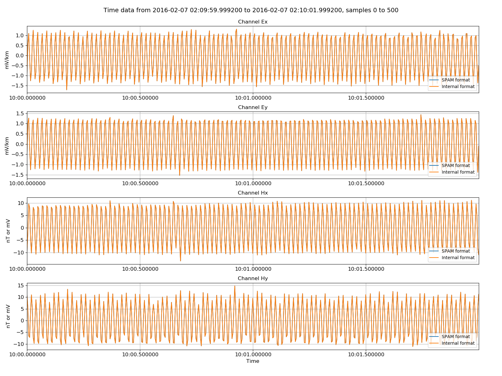
Original SPAM data versus the internally formatted data
There are a few helpful methods built in to resistics for manipulating timeseries data. These are generally in time. In the example below, the time data is band pass filtered between 0.2 Hz and 16 Hz.
47 48 49 50 51 | # all we see is 50Hz and 16Hz noise - apply a band pass filter
from resistics.time.filter import bandPass
filteredSPAMData = bandPass(physicalSPAMData, 0.2, 16, inplace=False)
filteredSPAMData.printInfo()
|
Printing the new time data information using filteredSPAMData.printInfo() now includes the application of the filter in the time data comments.
1 2 3 4 5 6 7 8 9 10 11 12 13 14 15 16 17 18 19 20 21 22 | 14:28:39 TimeData: ####################
14:28:39 TimeData: TIMEDATA INFO BEGIN
14:28:39 TimeData: ####################
14:28:39 TimeData: Sampling frequency [Hz] = 250.0
14:28:39 TimeData: Sample rate [s] = 0.004
14:28:39 TimeData: Number of samples = 300001
14:28:39 TimeData: Number of channels = 4
14:28:39 TimeData: Channels = ['Ex', 'Ey', 'Hx', 'Hy']
14:28:39 TimeData: Start time = 2016-02-07 02:09:59.999200
14:28:39 TimeData: Stop time = 2016-02-07 02:29:59.999200
14:28:39 TimeData: Comments
14:28:39 TimeData: Unscaled data 2016-02-07 02:09:59.999200 to 2016-02-07 02:29:59.999200 read in from measurement timeData\spam, samples 1949999 to 2249999
14:28:39 TimeData: Data read from 1 files in total
14:28:39 TimeData: Data scaled to mV for all channels using scalings in header files
14:28:39 TimeData: Sampling frequency 250.0
14:28:39 TimeData: Dividing channel Ex by electrode distance 0.0587 km to give mV/km
14:28:39 TimeData: Dividing channel Ey by electrode distance 0.0564 km to give mV/km
14:28:39 TimeData: Remove zeros: False, remove nans: False, remove average: True
14:28:39 TimeData: Band pass filter applied with cutoffs 0.2 Hz and 16 Hz
14:28:39 TimeData: ####################
14:28:39 TimeData: TIMEDATA INFO END
14:28:39 TimeData: ####################
|
It is possible to write out a modified time data object in internal (or ASCII) format. To do this, instead of using,
writer.writeDataset(spamReader, physical=True)
which writes out a whole dataset given a TimeReader object, use
writer.writeData(spamReader.getHeaders(), chanHeaders, filteredSPAMData, physical=True)
to write out a dataTimeData object directly. Header information needs to be explicitly passed to this function. For more information, see the example below and TimeWriter>. In the below example, the filtered time data is written out.
53 54 55 56 57 | # write out a filtered data - this is a subset of the data
spam_2filteredSubset = timePath / "spamInternalFiltered"
writer.setOutPath(spam_2filteredSubset)
chanHeaders, chanMap = spamReader.getChanHeaders()
writer.writeData(spamReader.getHeaders(), chanHeaders, filteredSPAMData, physical=True)
|
Opening the comments file for the newly written dataset, it can be seen that a line has been added which records the application of a filter to the dataset.
1 2 3 4 5 6 7 8 9 10 | Unscaled data 2016-02-07 02:09:59.999200 to 2016-02-07 02:29:59.999200 read in from measurement E:\magnetotellurics\code\resisticsdata\formats\timeData\spam, samples 1949999 to 2249999
Data read from 1 files in total
Data scaled to mV for all channels using scalings in header files
Sampling frequency 250.0
Dividing channel Ex by electrode distance 0.0587 km to give mV/km
Dividing channel Ey by electrode distance 0.0564 km to give mV/km
Remove zeros: False, remove nans: True, remove average: True
Band pass filter applied with cutoffs 0.2 Hz and 16 Hz
Time series dataset written to E:\magnetotellurics\code\resisticsdata\formats\timeData\spamInternalFiltered on 2019-10-05 18:15:29.301430 using resistics 0.0.6.dev2
---------------------------------------------------
|
Finally, to check everything is fine with the new dataset, the internal formatted filtered dataset can be read in and the data compared to the original filtered time data.
59 60 61 62 63 64 65 66 67 68 69 70 71 72 73 74 75 76 | # let's try reading in again
internalReaderFiltered = TimeReaderInternal(spam_2filteredSubset)
internalReaderFiltered.printInfo()
internalReaderFiltered.printComments()
# get the internal formatted filtered data
filteredInternalData = internalReaderFiltered.getPhysicalSamples()
filteredInternalData.printInfo()
# plot this against the original
fig = plt.figure(figsize=(16, 3 * physicalSPAMData.numChans))
filteredSPAMData.view(fig=fig, sampleStop=5000, label="filtered SPAM format")
filteredInternalData.view(
fig=fig, sampleStop=5000, label="filtered internal format", legend=True
)
fig.tight_layout(rect=[0, 0.02, 1, 0.96])
plt.show()
fig.savefig(timeImages / "spam_vs_internal_filtered.png")
|
Plotting the two time data objects on the same plot results in the image below.

Filtered SPAM data versus the internally formatted filtered data
Complete example script
For the purposes of clarity, the complete example script is shown below.
1 2 3 4 5 6 7 8 9 10 11 12 13 14 15 16 17 18 19 20 21 22 23 24 25 26 27 28 29 30 31 32 33 34 35 36 37 38 39 40 41 42 43 44 45 46 47 48 49 50 51 52 53 54 55 56 57 58 59 60 61 62 63 64 65 66 67 68 69 70 71 72 73 74 75 76 | from datapaths import timePath, timeImages
from resistics.time.reader_spam import TimeReaderSPAM
# read in spam data
spamPath = timePath / "spam"
spamReader = TimeReaderSPAM(spamPath)
spamReader.printInfo()
# get physical data from SPAM
import matplotlib.pyplot as plt

startTime = "2016-02-07 02:10:00"
stopTime = "2016-02-07 02:30:00"
physicalSPAMData = spamReader.getPhysicalData(startTime, stopTime, remnans=True)
physicalSPAMData.printInfo()
fig = plt.figure(figsize=(16, 3 * physicalSPAMData.numChans))
physicalSPAMData.view(fig=fig, sampleStop=2000)
fig.tight_layout(rect=[0, 0.02, 1, 0.96])
plt.show()
fig.savefig(timeImages / "spam.png")
# write out as the internal format
from resistics.time.writer_internal import TimeWriterInternal

spam_2internal = timePath / "spamInternal"
writer = TimeWriterInternal()
writer.setOutPath(spam_2internal)
writer.writeDataset(spamReader, physical=True)
# read in the internal format dataset and see what's in the comments
from resistics.time.reader_internal import TimeReaderInternal

internalReader = TimeReaderInternal(spam_2internal)
internalReader.printInfo()
internalReader.printComments()
physicalInternalData = internalReader.getPhysicalData(startTime, stopTime)
physicalInternalData.printInfo()

# now plot the two datasets together
fig = plt.figure(figsize=(16, 3 * physicalSPAMData.numChans))
physicalSPAMData.view(fig=fig, sampleStop=500, label="SPAM format")
physicalInternalData.view(fig=fig, sampleStop=500, label="Internal format", legend=True)
fig.tight_layout(rect=[0, 0.02, 1, 0.96])
plt.show()
fig.savefig(timeImages / "spam_vs_internal.png")
# all we see is 50Hz and 16Hz noise - apply a band pass filter
from resistics.time.filter import bandPass

filteredSPAMData = bandPass(physicalSPAMData, 0.2, 16, inplace=False)
filteredSPAMData.printInfo()
# write out a filtered data - this is a subset of the data
spam_2filteredSubset = timePath / "spamInternalFiltered"
writer.setOutPath(spam_2filteredSubset)
chanHeaders, chanMap = spamReader.getChanHeaders()
writer.writeData(spamReader.getHeaders(), chanHeaders, filteredSPAMData, physical=True)
# let's try reading in again
internalReaderFiltered = TimeReaderInternal(spam_2filteredSubset)
internalReaderFiltered.printInfo()
internalReaderFiltered.printComments()

# get the internal formatted filtered data
filteredInternalData = internalReaderFiltered.getPhysicalSamples()
filteredInternalData.printInfo()

# plot this against the original
fig = plt.figure(figsize=(16, 3 * physicalSPAMData.numChans))
filteredSPAMData.view(fig=fig, sampleStop=5000, label="filtered SPAM format")
filteredInternalData.view(
    fig=fig, sampleStop=5000, label="filtered internal format", legend=True
)
fig.tight_layout(rect=[0, 0.02, 1, 0.96])
plt.show()
fig.savefig(timeImages / "spam_vs_internal_filtered.png")
|